R bindings to H3, a hexagon-based geographic grid system via h3-js.
R bindings via native H3 C library can be found at h3r. h3r is much faster but requires installing h3 separately.
WARNING Functions do not support vectorized operations currently. The return value of vectorized input is unspecified. You should map over vectorized input instead.
Installation
You can install the released version of h3js from CRAN with:
Development version can be installed with:
Core functions
library(h3js)
library(sf)
library(tidyverse)

# Convert a lat/lng point to a hexagon index at resolution 7
h3_index <- h3_geo_to_h3(37.3615593, -122.0553238, 7)
h3_index
#> [1] "87283472bffffff"

# Get the center of the hexagon
hex_center_coordinates <- h3_to_geo(h3_index)
hex_center_coordinates
#> [1]   37.35172 -122.05033

# Get the vertices of the hexagon
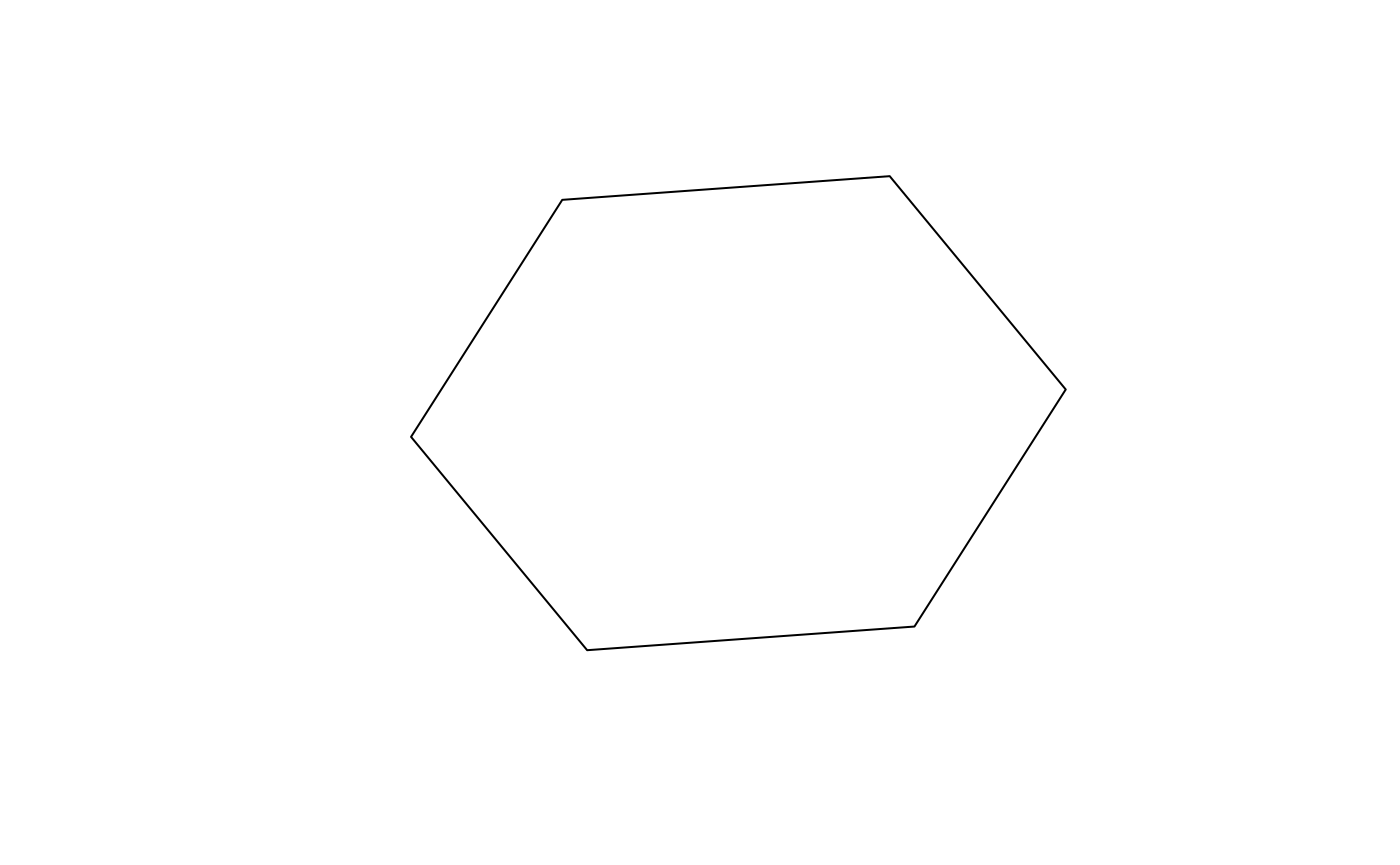
hex_boundary <- h3_to_geo_boundary(h3_index)
hex_boundary
#>          [,1]      [,2]
#> [1,] 37.34110 -122.0416
#> [2,] 37.35290 -122.0340
#> [3,] 37.36352 -122.0428
#> [4,] 37.36234 -122.0591
#> [5,] 37.35054 -122.0666
#> [6,] 37.33992 -122.0579

hex_boundary %>%
  # close polygon
  rbind(.[1,]) %>%
  # swap columns
  .[, c(2, 1)] %>%
  # convert to simple feature collection
  list() %>%
  st_polygon() %>%
  st_sfc() %>%
  plot()
Useful algorithms
# Get all neighbors within 1 step of the hexagon
h3_k_ring(h3_index, 1)
#> [1] "87283472bffffff" "87283472affffff" "87283470cffffff" "87283470dffffff"
#> [5] "872834776ffffff" "872834729ffffff" "872834728ffffff"

# Get the set of hexagons within a polygon
polygon <- list(
    c(37.813318999983238, -122.4089866999972145),
    c(37.7198061999978478, -122.3544736999993603),
    c(37.8151571999998453, -122.4798767000009008)
)
hexagons <- h3_polyfill(polygon, 7)
hexagons
#> [1] "872830828ffffff" "87283082effffff" "87283082affffff" "87283082bffffff"
#> [5] "872830876ffffff" "872830820ffffff" "872830870ffffff"

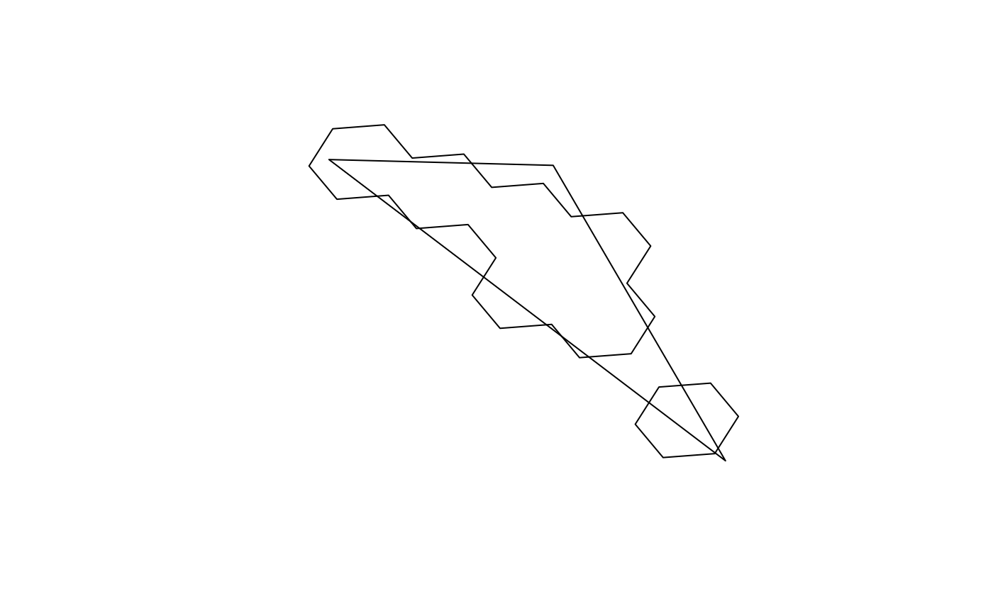
# Get the outline of a set of hexagons, as a GeoJSON-style MultiPolygon
coordinates <- h3_set_to_multi_polygon(hexagons, TRUE)

c(
  coordinates %>%
    map(~ matrix(.x, ncol = 2)) %>%
    map(list) %>%
    st_multipolygon() %>%
    st_sfc(),
  do.call(rbind, polygon) %>%
    # close polygon
    rbind(.[1,]) %>%
    # swap columns
    .[, c(2, 1)] %>%
    list %>%
    st_polygon() %>%
    st_sfc()
) %>%
  st_sf() %>%
  plot()
Benchmark
Houston <- list(lat = 29.7632836, lon = -95.3632715)

microbenchmark::microbenchmark(
  h3r::getIndexFromCoords(Houston$lat, Houston$lon, resolution = 5),
  h3_geo_to_h3(Houston$lat, Houston$lon, res = 5),
  h3r::getBoundingHexFromCoords(Houston$lat, Houston$lon, resolution = 5),
  h3_to_geo_boundary(h3_geo_to_h3(Houston$lat, Houston$lon, res = 5))
)
#> Unit: microseconds
#>                                                                     expr
#>        h3r::getIndexFromCoords(Houston$lat, Houston$lon, resolution = 5)
#>                          h3_geo_to_h3(Houston$lat, Houston$lon, res = 5)
#>  h3r::getBoundingHexFromCoords(Houston$lat, Houston$lon, resolution = 5)
#>      h3_to_geo_boundary(h3_geo_to_h3(Houston$lat, Houston$lon, res = 5))
#>       min        lq       mean    median        uq       max neval
#>    12.074   29.1875  142.95902   42.3495   60.9185  9666.731   100
#>   729.252 1065.5555 1725.82045 1501.5660 2151.0500  5801.808   100
#>    17.404   34.8925   56.74685   50.5785   59.7705   406.992   100
#>  1361.911 2132.8900 3377.73784 2801.3605 3811.4555 17681.988   100